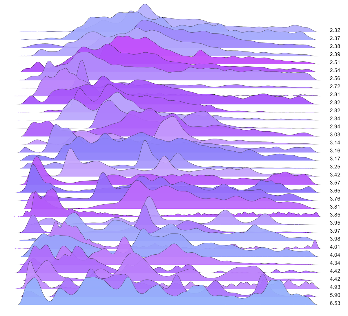
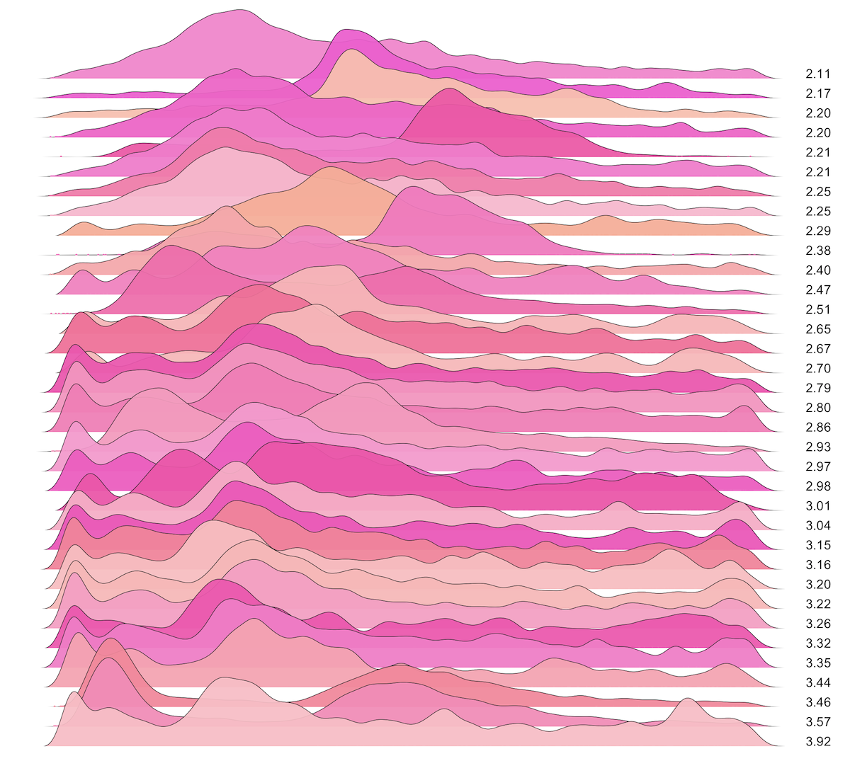
Frequency Trails: Modes and Modality
It is a truth universally acknowledged that the average is the index of central tendency. But what if the tendency isn't central?
I've worked many performance issues where the latency or response time was multimodal, and higher-latency modes turned out to be the cause of the problem. Their existence isn't shown by the average – the arithmetic mean; it could only be seen by examining the distribution as a histogram, density plot, heat map, or frequency trail. Once you know that more than one mode is present, it's often straightforward to determine what causes the slower mode, by seeing what parameters of the operations involved are different: their type, size, URL, code path, etc.
I previously visualized outliers, created a test for their detection, and then surveyed hundreds of production servers to quantify their occurrence. On this page I'll do the same for detecting multiple modes.
Visualization
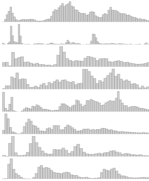
Disk I/O latency, 10,000 I/O, as a histogram:
The height of each column shows how many I/O occurred in the latency range (x-axis). The shape of this histogram shows two modes (peaks): one at 0 - 200 us, and another at 2.2 to 2.4 ms.
The same disk I/O latency as a frequency trail:
This is similar to the histogram, showing higher-resolution details for the modes, and the location of outliers as individual points.
By visualizing the distribution, it is easy to identify it as bimodal. The problem arises when you're faced with thousands of distributions, where an automatic test would be very helpful.
Problem
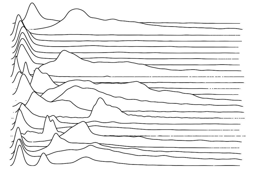
Here are disk I/O latency distributions from 25 servers, as a frequency trail waterfall plot:
One looks trimodal. Some look bimodal. And some look in between.
Detection
There are many proposed methods for detecting bimodal and multimodal distributions. For the same reasons explained in my page on outliers, we'd like this test to be as simple as possible, while tolerating false positives rather than false negatives.
To detect multiple modes, I'll use an indirect approach which calculates an mvalue (modal value) and compare this to a threshold.
mvalue
This sums the absolute differential of the frequency or probability distribution, where that may be a histogram of binned data or a sampled kernel density estimate, and then divides the sum by the maximum frequency or probability (density). The value is relative to the number and size (total probability) of the modes.
This can be expressed for the histogram, x, with bins, n (including zero bin terminators), and maximum bin value, M, the mvalue, m(x), is:
             1  n
      m(x) = -  ∑ |xi - xi-1|
             M i=2
The same expression is true for the kernel density estimate, x, with samples, n, and maximum density estimate, M.
This may be best explained by considering the following synthetic bimodal distribution:
The mvalue sums the absolute difference in elevation, normalized for the height of the plot. A unimodal distribution has an mvalue of 2: 1 for the rise to the peak, and another 1 for the fall back to zero. A bimodal distribution has an mvalue of 4, as shown in this picture.
Since the height is normalized to the highest peak, minor modes do not necessarily have the same height as the major mode, which results in fractional values for the mvalue. For example, consider a bimodal distribution with a minor mode that has half the probability of the major mode. The minor mode should have half the height of the major node, and an mvalue should be 3. The mvalue indicates the product of the size (volume) and number of modes.
UPDATE: The mvalue is pretty similar to total variation, first introduced by Camille Jordan [3][4].
Modal Test
A test can be performed by comparing the mvalue to a threshold which indicates that multiple modes may be present, and that the distribution should be investigated further (eg, using a visualization). My suggestion is the value 2.4; you can study the later waterfall plots to see what this will and won't detect, or to choose your own value. This threshold is similar to the role of "6" in the six sigma outlier test: it will err on the side of false positives, since the next action is to examine the full distribution to confirm or deny the finding.
Calculating mvalue
There are three tricks for calculating mvalues.
1) Outliers need to be trimmed. The following is the same distribution, with some outliers:
This merges the bulk of the data, reducing the change in elevation needed to identify the modes. This is much worse when implemented as a histogram, like that shown earlier, as both modes may be merged into one column.
Outliers can be trimmed by only including data within the range: Q1 – 1.5 x IQR to Q3 + 1.5 x IQR, similar to the range used by Tukey for box plots. A non-robust technique, but one that may be easier depending on what you have available, is to include data only within two standard deviations.
2) A series of bin sizes or bandwidths should be used for calculating mvalues, and the maximum mvalue used. For histograms, this means selecting a series of different bin sizes, then creating a histogram based on each, and taking the largest mvalue from the series of histograms. A similar approach can be used for kernel density estimates by varying the bandwidth.
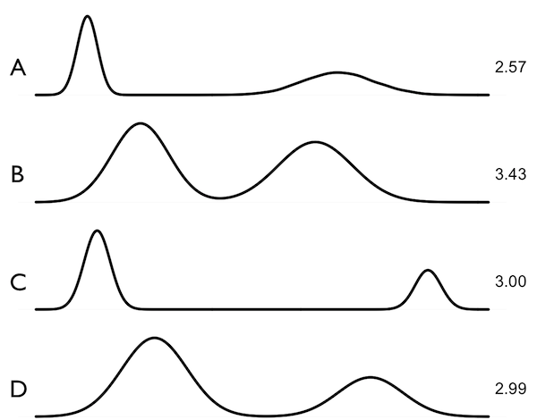
The problem this addresses is with multiple modes with different degrees of variance. Consider the density plots on the right. A) Shows a bimodal distribution where each mode is equal in numbers of samples, however, the right mode has a greater variance, lowering its height in this density plot, and lowering the mvalue to 2.57. This low height is an artifact of the small kernel density estimate bandwidth. B) shows the same distribution as (A), but with a much larger bandwidth (smoothing), which lowers the left mode, which raises the relative height of the right mode. This produces a higher mvalue, better matching the known distribution. C) is an example where the right mode has half the samples as the left, and the mvalue of 3.00 is expected. D) shows the same distribution as (C), with a greater bandwidth, which has not really changed the mvalue (good).
For histograms, a similar problem exists with wider variance minor nodes. By trying larger bin sizes (column widths), more samples are aggregated in each column, increasing the height of the minor mode columns, and better reflecting their size in the mvalue.
Other approaches to coalesce minor modes can be tried. This simple approach runs the risk of merging close modes, and under reporting their size in the mvalue.
3) The bin size or bandwidth must be carefully chosen: specifically, the smallest size from the series. It cannot be too small, or minor fluctuations will be included in the mvalue. Nor can it be so large as to merge multiple modes. This selection is subjective.
For some distribution types, it may also make sense to use a non-linear binning function, such as logarithmic, if the higher modes are expected to have greater variance. More on this in later sections.
Synthetic
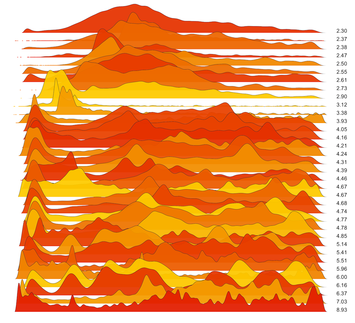
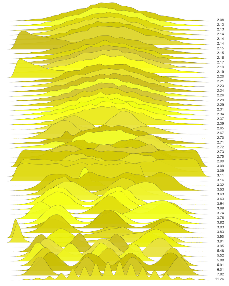
These are waterfall plots of overlapping frequency trails, with the mvalue on the right. Each is a synthetic distribution from a collection I'm using to test modality detection. Since these often overlap, I've randomly colored them for differentiation, and also added a little transparency here so that background detail can still be seen if you look carefully.
 |
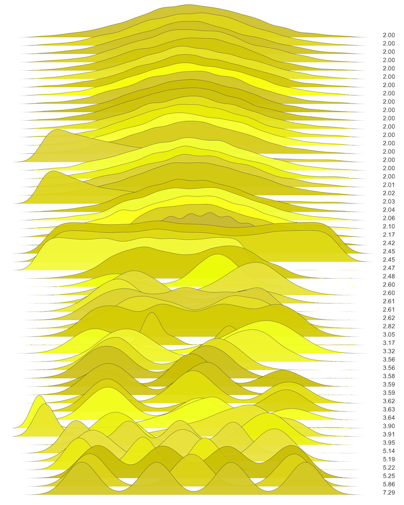 |
These plots are in ascending mvalue order, visualizing how the mvalue detects modality. The effect of kernel density bandwidth can also be compared: the left plots use a small minimum bandwidth, which inflates the mvalue due to small fluctuations, and the right plots use a larger minimum bandwidth, which smooths the plots and produces mvalues that better match the test distributions. The plots that follow use the best of both worlds: a smaller bandwidth for drawing the plot, and a larger minimum bandwidth for calculating the mvalue. All of these plots have had outliers trimmed.
The mvalue works well: at the top of the right plot are unimodal distributions with a sum of 2.0. At the bottom is a quadmodal distribution with an mvalue of 7.29, clearly indicating multiple modes.
Latency
Latency is time spent waiting, and is used here to refer to the entire time for I/O or service requests.
Disk I/O Latency
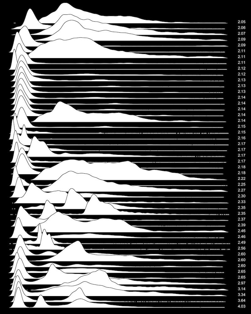
The following are disk I/O latency distributions from 50 random production servers. The latency was measured at the block device interface, and each distribution is composed of around 10,000 I/O. The mvalue is shown on the right.
 |
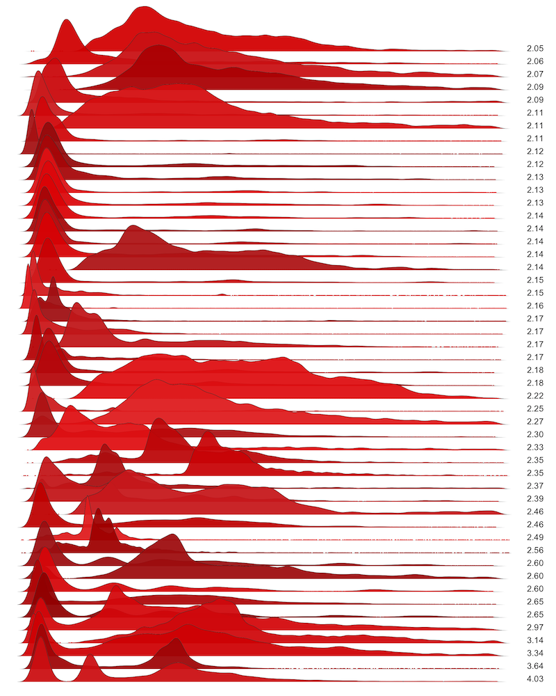 |
Inverted and colored versions are shown of the same data. Also see the 200 server version: using the modal test (2.4), 29% of these are multimodal.
MySQL Latency
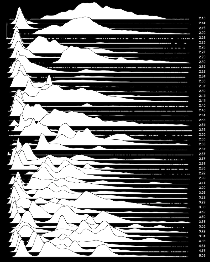
Here is MySQL command latency from 50 random production servers, showing around 10,000 commands for each distribution:
 |
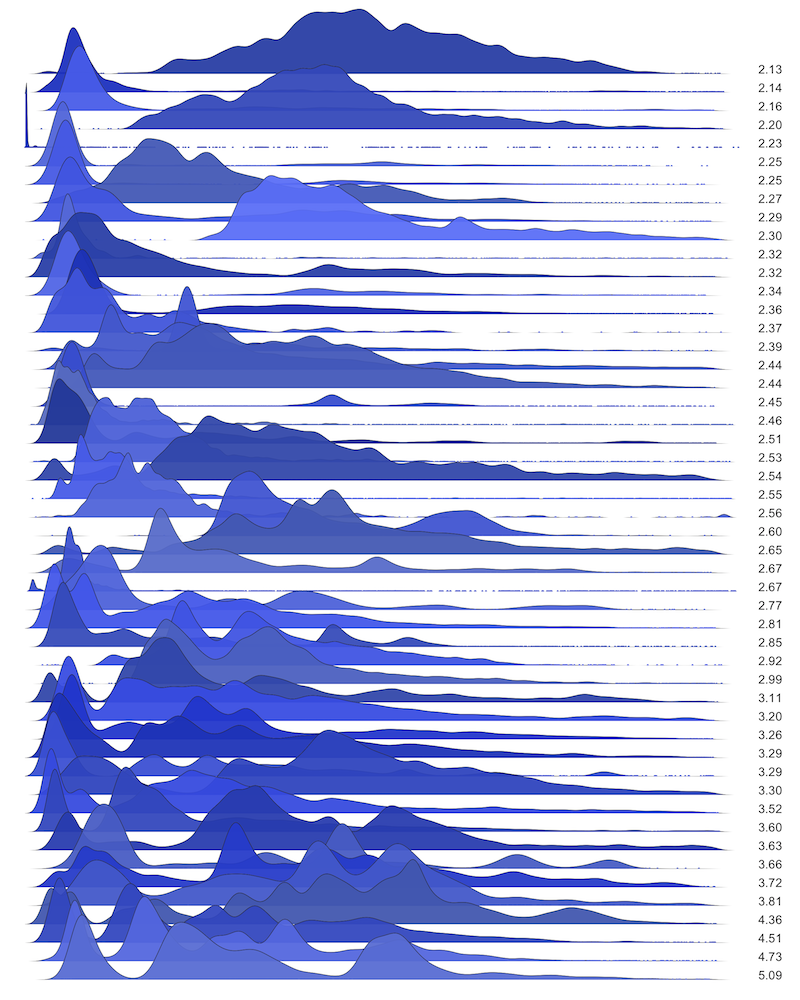 |
Also see the 100 server version: using the modal test (2.4), 72% of these are multimodal.
node.js Latency
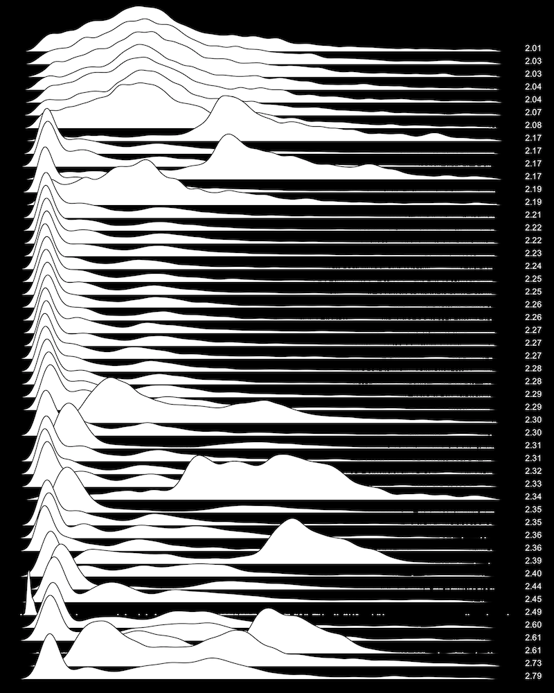
Here is node.js HTTP server response time (latency) from 50 random production servers, showing around 10,000 responses each:
 |
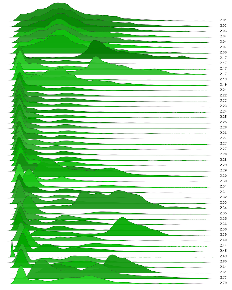 |
Also see the 200 server version: using the modal test (2.4), 20% of these are multimodal.
Latency Cost
Latency distributions have a characteristic not captured by the previous distribution plots: slower operations have a higher cost than faster operations.
Consider a bimodal distribution composed of eleven I/O: 10 at 1 ms, and 1 at 10 ms. This will have a mvalue of 2.2, as the second mode has one tenth the frequency of the first. However, the cost to synchronously block on the I/O can be described as: "fast I/O" totaling 10 ms (10 x 1), and "slow I/O" totaling 10 ms (1 x 10). The fast and slow modes cost the same.
This can be reflected by weighting each I/O with its latency (something I learned from Bryan, who developed it as a colorization method for latency heat maps). This multiplies the distribution plot by the x-axis value. This example distribution would then have a latency cost mvalue of 4, as each mode has the same height (10 ms).
If you look back at the earlier disk I/O waterfall plot, there are many distributions with a very low major mode (disk cache hits), and a smaller and wider minor mode (disk cache misses). Accounting for latency cost, these minor modes will be magnified, and may cost more than the major mode.
Disk I/O Cost
The following are disk I/O latency cost distributions, from 35 servers (same pool as shown before). More hues have been used here to differentiate the more frequent overlaps.
This better matches my experience debugging disk I/O performance issues. They are often caused by the slower disk I/O mode, even if it is a fraction of the frequency when compared to the disk cache hit mode, because it has a much higher cost.
Using the modal test (2.4), 91% of these are multimodal.
MySQL Cost
MySQL command latency cost distributions, from 35 servers (same pool as shown before):
Using the modal test (2.4), 89% of these are multimodal.
Node.js Cost
Node.js HTTP server response time cost distributions, from 35 servers (same pool as shown before):
Using the modal test (2.4), 71% of these are multimodal.
What Causes Multiple Modes?
Separate modes can be caused by many factors. Examples for latency modes:
- fast path / slow path: Applications and the kernel often have performance optimizations for common operations, where slower code can be bypassed with faster code: the "fast path". Each path has different latency characteristics, creating different modes in the distribution. I've debugged tons of these: eg, IPv4 having fast paths in the kernel that IPv6 doesn't have; the presence of VLAN tags causing packets to take the slow path; etc.
- cache hit / cache miss: Caches hits and misses are separate latency modes, and caches are commonly used throughout applications, the kernel, and hardware. There can be over ten levels of cache between an application request and disk I/O, including an application cache, a database cache, a file system inode cache, a file system data cache, a second level of cache (flash), a file system device cache, the block cache (buffer cache), a physical disk controller cache, a storage array cache, and finally the disk cache. Each creates its own mode for cache hits.
- small I/O / large I/O: Small I/O is usually faster to perform than large I/O, at the very least due to the extra clock cycles to move main memory.
- sync / asynch: Synchronous vs asynchronous I/O, or non-blocking I/O, will cause different modes. Synchronous file system writes should block on disk I/O latency, waiting until the data has been flushed to permanent storage. Asynchronous I/O does not wait.
- request type: Application requests may have different costs to perform, which show as different latency modes. Unlike fast path / slow path, which is an implementation detail, different request types may be part of the API, and always expected to respond with different latency. For example, the latency to view a web page may be one mode, and the latency to post a comment another.
Implementing the Modal Test
The latency measurements used here were traced using DTrace, and then post-processed using R.
The mvalue can be implemented by these steps:
- Remove outliers from data.
- Select the smallest bin size.
- Group data into equally sized bins for the range.
- Step through bins, summing the absolute difference in bin counts, adding terminator bins of zero.
- Calculate mvalue: divide sum by largest bin count.
- Select a larger bin size.
- Goto 3, and repeat until largest bin size tried.
- Use the largest mvalue found.
The modal test then tests if this value is greater than or equal to 2.4.
Here are some example calculations from the process:
-
Step 3: the histogram has the following bin counts: 17, 0, 0, 0, 3, 4, 2, 0.
Step 4: the sum is: 17 (|17 - 0|) + 17 (|0 - 17|) + 0 (|0 - 0|) + 0 (|0 - 0|) + 3 (|3 - 0|) + 1 (|4 - 3|) + 2 (|2 - 4|) + 2 (|0 - 2|) + 0 (|0 - 0|) = 42.
Step 5: the highest bin count is 17, so the mvalue = 42 / 17 = 2.47.
Step 6: the bin size is increased. Eg, by doubling it.
Step 3: the histogram now has the following bin counts: 17, 0, 7, 2.
Step 4: the sum is: 17 (|17 - 0|) + 17 (|0 - 17|) + 7 (|7 - 0|) + 5 (|2 - 7|) + 2 (|0 - 2|) = 48.
Step 5: the highest bin count is 17, so the mvalue = 48 / 17 = 2.82.
Step 6: the bin size is increased. Eg, by doubling it.
Step 3: the histogram now has the following bin counts: 17, 9.
Step 4: the sum is: 17 (|17 - 0|) + 8 (|9 - 17|) + 9 (|0 - 9|) = 34.
Step 5: the highest bin count is 17, so the mvalue = 34 / 17 = 2.00.
Step 6: no more bin sizes to try.
Step 8: largest mvalue found = 2.82.
This can be implemented a variety of ways. Outlier removal may be based on IQR as described earlier, mean +- 2σ, or based on a trusted threshold for the given distribution. The minimum bin size can be picked based on the smallest separation desired for identifying modes. Binning data, as visualized by histograms, is easier to implement and use than a kernel density estimate.
As a simple example, let's say that operations are expected to be between 0 and 100 ms. Outlier removal can then implemented by discarding measurements beyond 100 ms. Binning can be implemented by picking a size suitable for the range and desires for mode detection: eg, a 1 ms bin size to detect modes separated by at least 1 ms, which divides the range into a 100-element array. This filtering and binning can be performed in real time as the operations complete. You can later vary bin size to find the maximum mvalue, by coalescing the 1 ms bins.
Example Implementation
As an example, the following DTrace program prints a power-of-2 histogram of disk I/O latency every second, and pipes this to to awk, which calculates and adds the modal count beneath the DTrace histograms. This histogram type is better suited for this latency distribution, as the higher latency modes have higher variance, and the power-of-2 binning naturally groups them together.
# dtrace -qn 'io:::start { ts[arg0] = timestamp; }
    io:::done /ts[arg0]/ {
	@ = quantize((timestamp - ts[arg0]) / 1000); ts[arg0] = 0; }
    tick-1s { printa("\ndisk I/O (us):%@dDONE\n", @); trunc(@); }' | awk '
    $3 ~ /^[0-9]/ { s += ($3 - l) > 0 ? $3 - l : l - $3;
	if ($3 > m) { m = $3 } l = $3; }
    { if ($1 == "DONE") { printf "mvalue: %.2f\n", s / m; s = m = l = 0; }
	else { print $0 } }'

disk I/O (us):
           value  ------------- Distribution ------------- count
              16 |                                         0
              32 |@@@                                      12
              64 |@@@@@@@@@@@@@@                           56
             128 |@@@@@@@@@@@@@@@@                         67
             256 |@@@@@@                                   23
             512 |@@                                       7
            1024 |                                         0
mvalue: 2.00

disk I/O (us):
           value  ------------- Distribution ------------- count
              64 |                                         0
             128 |@@@@@@@@@@@@@@@                          42
             256 |@@@@@                                    13
             512 |                                         1
            1024 |@@                                       5
            2048 |@@@@@                                    14
            4096 |@@@@@@@@@@@@@                            37
            8192 |@                                        2
           16384 |                                         0
mvalue: 3.71

disk I/O (us):
           value  ------------- Distribution ------------- count
              16 |                                         0
              32 |                                         1
              64 |@@@@@@@@@@                               35
             128 |@@@@@@@@@@@@@@@@@@@@@                    76
             256 |@                                        4
             512 |@                                        3
            1024 |@@                                       8
            2048 |@@@@@                                    19
            4096 |                                         0
mvalue: 2.42
[...]
This is a simple implementation which does not vary the bin size, so it may produce low mvalues for wider minor modes.
About mvalues
The mvalue and the modal test presented here are one way to detect multiple modes, and is an indirect approach: it doesn't seek to find the modes directly (the local maximums).
Strengths:
- Relatively easy and intuitive.
- Reflects modes linearly: increasing equally sized modes produce mvalues of 2, 4, 6, ...
- Produces fractional values for smaller minor modes, allowing fractional thresholds to be used as a modal test.
Weaknesses:
- More computation than simple statistics. Requires binning of data, or a kernel density estimate.
- Sensitive to the minimum bin size or bandwidth used, for accurate detection.
- Struggles to accurately detect close modes with either overlapping functions or where one mode has much wider variance: eg, a major node with a close and wide minor node. Using a series of larger bin sizes or bandwidths is used to find the wider variance modes, however, if they are close to other modes they can overlap and be included in the same bin. This results in an mvalue smaller than it should be. Latency is a special case, where many distributions have a low-latency major node and a closer higher-latency minor node with large variance: which which may bin better when using a logarithmic scale, like the DTrace example earlier.
Bear in mind that the role of mvalues is a means to an end, but not the end itself. They can be used with a modal test, using a threshold (2.4), to indicate that a distribution is worth investigating further: such as by using a visualization.
Other Tests
I'd prefer a simpler test for multiple modes, but haven't yet found one that is reliable. I have investigated using various statistical properties in different ways for this, including CoV, MAD, percentiles, IQR, skewness, kurtosis, as well as other statistical tests, without real success.
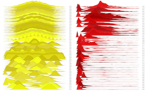
The bimodality coefficient for a finite sample is pictured on the right for synthetic and disk distributions, with the bimodality coefficient value on the right of each, so that you can visualize what each value identifies. Considering both synthetic and real distributions, the value doesn't satisfactorily reflect modality.
I found the Shapiro-Wilk test to be very good at identifying normal and not-normal distributions; however, many unimodal distributions are not normal: latency distributions often have a tail and positive skewness. I also tried the Anderson-Darling Goodness of Fit test, and the Kolmogorov-Smirnov test.
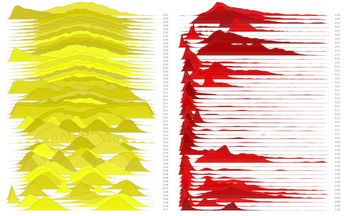
The diptest is shown on the right, for both synthetic and disk distributions, with the diptest value on the right of each. Like the bimadality coefficient, this showed promise, but didn't satisfactorily identify multiple modes. The largest diptest value for the synthetic distributions is bimodal, with a higher diptest value than the trimodal and quadmodal distributions. Although, the diptest appears to account for the distance between modes – something that the mvalue and modal test does not.
There are also direct approaches for counting the modes, or local maximums, in the distribution. These don't account for the size of the modes, like mvalues, but counts them instead. These approaches may inflate the mode count if perturbations are detected as modes, however, given a tolerance for false positives rather than false negatives, this may be acceptable. As with the mvalue, the next step should be to examine the distribution anyway, to confirm the findings.
The best test of all is a visualization: a histogram, density plot, heat map, or frequency trail.
Conclusion
Multiple modes can be detected by measuring the change in elevation of the frequency or probability distribution, which may be a histogram or kernel density estimate. The value is then normalized by dividing by the largest frequency or probability value. This produces an mvalue of 2 for a normal distribution: 1 for the rise to the peak, and 1 for the fall back to zero. An evenly-divided bimodal distribution has an mvalue of 4, and higher numbers of modes have higher mvalues. A modal test compares this to a threshold, such as 2.4, for identifying distributions that may be multimodal and worth investigating further.
For the mvalue calculation to be reliable, outliers must first be trimmed from the data. Selection of the histogram bin size (or density bandwidth) is important: too-small and subtle variations inflate the mvalue; too-large and multiple modes can be missed (merged). Different bin sizes (or a way to coalesce bins) should be tried for the same distribution, to fairly identify multiple modes which have different variance, and for which a small bin size will unfairly reduce the height of the larger variance modes.
With its sensitivity to bin size and bin division points for fairly reflecting the size of the modes, as well as the computation required, this is not a perfect approach for mode detection. It's one approach that has been explored here, and is an indirect approach for mode detection.
I visualized synthetic distributions with varying modes to show what the mvalue represents, then used this on real-world distributions of three types of latency: disk I/O, MySQL, and node.js, from over one hundred production servers. Between 20% and 72% of the surveyed distributions were multimodal based on a 2.4 mvalue test.
Latency cost distributions were also identified, which weights slower operations with their latency cost. For the latency distributions sampled, at least 71% of them were multimodal when accounting for latency cost.
Understanding multiple modes is important for performance analysis, especially for latency distributions. The average, or mean, implies a central tendency, which is often not the case.
References, Acknowledgements
Resources:
- [Rice 95] Rice, J. Mathematical Statistics and Data Analysis, 2nd Ed., Duxbury Press
- [1] http://en.wikipedia.org/wiki/Multimodal_distribution
- [2] http://en.wikipedia.org/wiki/Probability_density_function
- [3] http://en.wikipedia.org/wiki/Total_variation
- [4] http://www.encyclopediaofmath.org/index.php/Function_of_bounded_variation#Historical_remark
Thanks to those who sent feedback on this and gave me suggestions for future work in this area, including Theo Schlossnagle, Matt Smillie, Robert Mustacchi, Baron Schwartz, and Heinrich Hartmann. And thanks to Deirdré Straughan for edits!
For more frequency trails, see the main page. For the next part in this series, see mean.
Updates
- 2020: Andrey Akinshin has developed a new approach with better mode detection accuracy, based on studying the valleys rather than the peaks: see Lowland multimodality detection.
